Utilizing artificial intelligence to forecast pulmonary hemorrhage in premature infants
Setting
This retrospective study was conducted at Cleveland Clinic Children’s Hospital, which has two level 3 and one level 4 neonatal intensive care units (NICUs) with approximately 10,000 deliveries annually.
Patients
The study included all infants with gestational age (GA) < 32 weeks and/or birth weight (BW) < 1500 g who had a documented diagnosis of PHEM. For each case with PHEM, 2 controls were selected who were born in the same year, were chronologically closest to the case, had the same week of GA, and had a BW within 50 g of the case. The study utilized data from January 1st, 2013, through December 31st, 2021. Hemorrhage was diagnosed if significant bleeding was found in the airways that necessitated considerable escalation of respiratory support. Infants with blood-tinged secretions in the endotracheal tubes were not diagnosed with PHEM. Given the pilot nature of the study and the rarity of the disease, power analysis was not applicable; however, the study included all available cases with PHEM over a span of 9 years.
Delivery room management
Delivery rooms were staffed by maternal-fetal medicine specialists and in-house neonatologists. Delayed cord clamping (>30 s) was routinely practiced for all deliveries, unless deemed unfeasible. A change in neonatal resuscitation practices occurred during the study period. Prior to 2019, all extreme preterm infants were routinely intubated and administered surfactant. After 2019, guidelines were revised to favor initial resuscitation with continuous positive airway pressure (CPAP) in the delivery room, except for periviable non-vigorous preterm infants, followed by bubble CPAP upon NICU admission. No other significant changes were recalled regarding the use of prenatal steroids, magnesium sulfate, or postnatal caffeine.
Data management
Electronic medical records (EMR) were retrieved, and multiple maternal and neonatal variables were collected. Maternal data included age, race, parity, presence of gestational hypertension, presence of chorioamnionitis, platelet count on the day of delivery, timing of amniotic membrane rupture, antepartum steroid administration, and use of magnesium prophylaxis. Infant data collected included Apgar scores at 1 and 5 minutes, sex, BW, mode of birth, and delivery room resuscitation measures (intubation, chest compression, and the use of epinephrine). Clinical and laboratory data were collected in 12-hour epochs for the first 72 hours or until PHEM occurred. The data in each epoch included three values for each following variable: heart rate, blood pressure, fraction of inspired oxygen (FiO2), and measured blood gas components. The three values represented the mean, lowest, and highest values during each 12-hour period. Mode of ventilation, complete blood count, surfactant administration, fluid intake, and use of caffeine were all recorded.
Statistical analysis
Continuous variables were summarized with mean (M) and standard deviation (SD) or medians (MED) and interquartile ranges (IQR) and compared using T tests or the Mann–Whitney U test. Categorical variables were reported with frequencies and percentages and compared using chi-squared tests. A p value < 0.05 was considered significant.
AI model training
Data processing
Data pre-processing involved encoding categorical variables, handling missing values, and normalizing continuous variables to ensure model compatibility. Infants were stratified into categories based on BW (<700, 700–1000, and >1000 g) and GA (<25 weeks, 25–27 weeks, and >27 weeks). To achieve maximum accuracy, we eliminated infants with missing data for training the AI model. Continuous variables were entered into the model after being categorized into nominal variables. For instance, arterial blood pressure values within each epoch were categorized into 3 categories: 0, 1 & 2. These categories were assigned based on the lowest quartile, middle half, and highest quartile of all values. Consequently, within each 12-hour epoch, blood pressure in the lowest 25th percentile would receive a score of 0, while the highest 25th percentile readings and the mean may receive scores of 2 or 1 based on the actual blood pressure measurement. Similar approaches were employed for heart rate, oxygen requirement, and blood gas parameters. It is important to note that these scores were generated solely for the purpose of the model and did not necessarily reflect clinical diagnoses such as hypotension, tachycardia, or acidemia. A list of categorized variables is provided in the supplemental table.
Model training
A random forest algorithm was employed for model training due to its robustness, ability to handle both categorical and continuous variables, and strong performance in medical prediction tasks. The Random Forest algorithm is an ensemble machine learning method that builds multiple decision trees during training and aggregates their results to improve prediction accuracy and generalizability [7]. Each tree is trained on a random subset of the data and a random subset of features, which helps reduce overfitting and variance. This approach can be likened to consulting multiple independent experts—each providing an opinion based on different evidence—and then combining their responses to reach a consensus, which often yields a more reliable decision than relying on a single opinion. Each “expert” is, in fact, a decision tree. A forest is a collection of these decision trees. The trees are built randomly and independently, hence the name: Random Forest.
Random Forest was selected for this study due to its robustness in handling high-dimensional data, its ability to model complex, non-linear relationships, and its resilience against overfitting and outliers [7, 8]. Moreover, it provides useful measures of feature importance, which are valuable for interpreting model results. These characteristics make Random Forest a suitable and effective choice for our dataset, which includes diverse and potentially noisy features.
In this study, the model was trained on 90 patient records using 80 decision trees (estimators), with each tree allowed a maximum depth of 15 decision nodes, a parameter that controls model complexity and helps avoid overfitting. For instance, in predicting respiratory distress, one decision tree might split data based on gestational age, birth weight, and Apgar score, while others utilize different combinations. To ensure reliability, we applied 10-fold cross-validation within the training dataset. This technique partitions the data into 10 subsets, using nine for training and one for validation, rotating through all subsets. This improves generalizability and minimizes the risk of overfitting.
Model evaluation
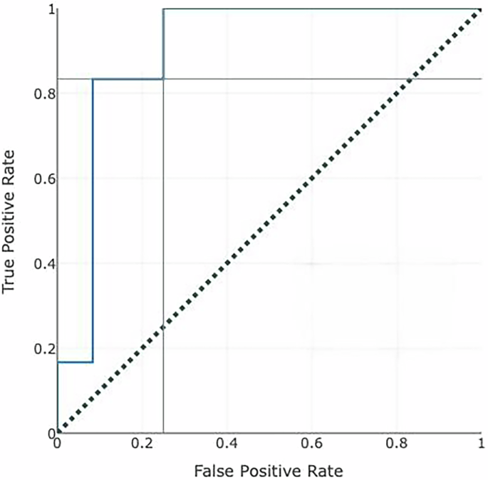
The performance of the trained model was evaluated using a separate holdout test set, ensuring an unbiased evaluation of the model’s predictive power in real-world scenarios. Model discrimination was assessed using the area under the receiver operating characteristic curve (AUC-ROC), while calibration—the agreement between predicted probabilities and observed outcomes—was evaluated using a calibration plot. The calibration curve was generated by plotting predicted probabilities against observed outcome frequencies using a LOESS smoothing function, with a 45-degree reference line indicating perfect calibration. Calibration slope and intercept were also calculated to assess model fit. Internal validation was performed using cross-validation within the training dataset to mitigate the risk of overfitting.
Lift curve construction and interpretation: Patients were ranked in descending order by their predicted probability of pulmonary hemorrhage. The lift curve plots the cumulative proportion of patients flagged (x-axis) against the proportion of true positive cases captured (y-axis), following the approach described by Powers (2015) [9]. This ordering ensures that the curve reflects the model’s ability to prioritize high-risk cases. The area under the precision-recall curve (AUPRC) and related metrics were also assessed.
In this case–control design, hemorrhage prevalence was 33% (1 case per 2 controls). Therefore, randomly selecting 33% of patients would yield 33% of true positives by chance. This diagonal “baseline” or “chance” line in the lift plot represents the expected performance of a non-informative model. Our model’s performance exceeds this baseline—at the 0.50 cutoff, for example, it captures approximately 71% of true positives compared to 33% expected by chance (lift = 2.1).